Analyse
Measurements
Load real observations, find their station, and compare them with the simulation.
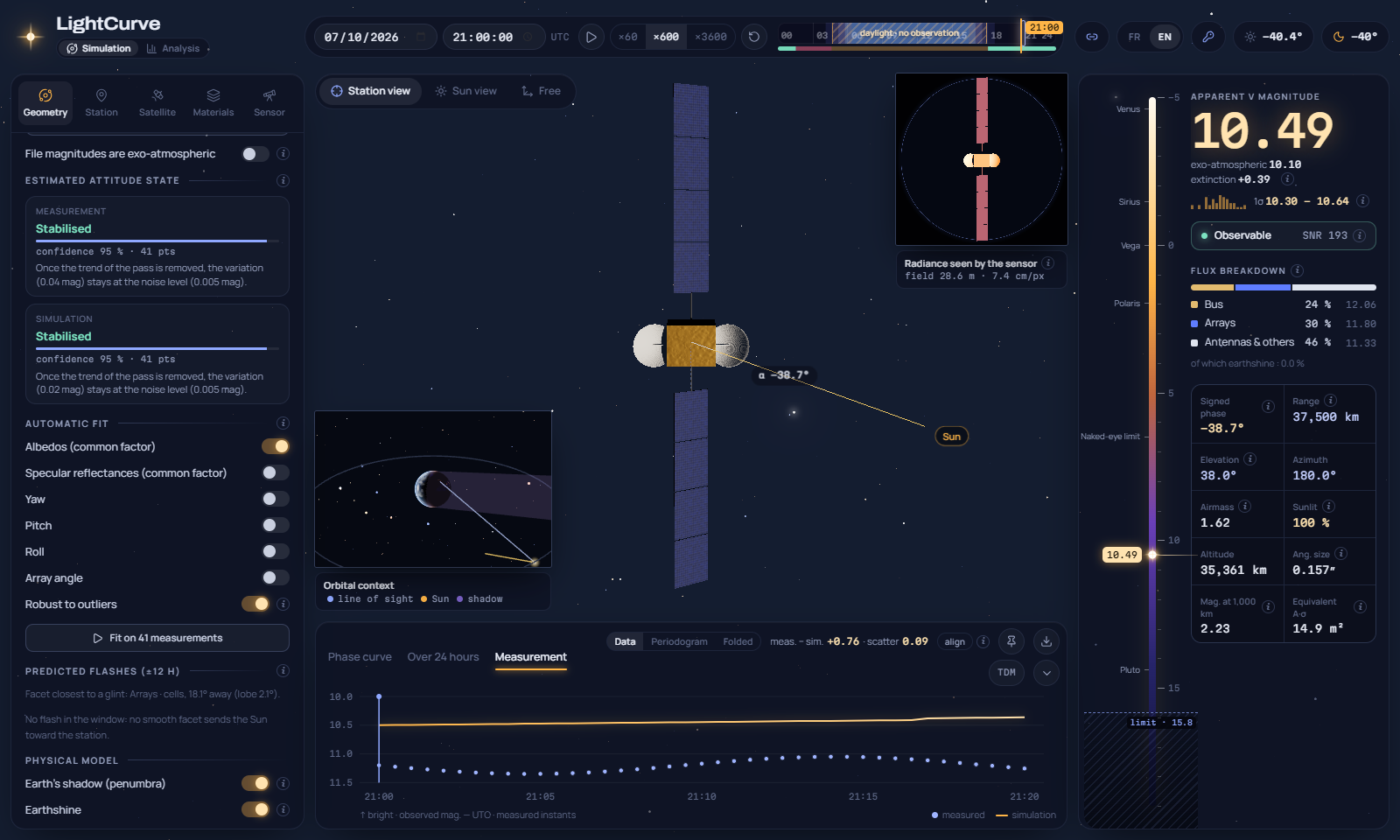
Load observations
Section titled “Load observations”In the Geometry tab.
Add a file appends the series of another file — other nights, other stations — for a joint fit.
The scene follows the measured line of sight, interpolated between measurements; the period appears on the timeline. A slider moves within the measurement.
Where was the station?
Section titled “Where was the station?”| Source | When |
|---|---|
| A stations file (format) | The measurement names a station listed in it |
| Recovered from the angles | The file gives both RA/Dec and azimuth/elevation: least squares on latitude and longitude, trying J2000 and of-date RA/Dec; the altitude is taken from the nearest known site within 5 km |
With both, the angles serve as a check (distance in km). On a real 60-point series of a geostationary object, the station was recovered within 0.5 km of its true position.
Compare
Section titled “Compare”The Measurement curve plots the measured magnitudes (points) and the simulated ones (line), with:
| Statistic | Meaning |
|---|---|
| meas. − sim. | Mean difference. Positive: the real object is fainter than the model |
| scatter | Standard deviation once the mean difference is removed: agreement of the shape |
| Δphase | Mean difference between the phase angle of the file and the recomputed one: close to 0, it confirms the station and geometry |
Align shifts the simulated curve by the mean difference to compare shapes. The magnitudes of the file are compared with the observed magnitude (extinction included), or with the exo-atmospheric one if you say so.